Botulism Data

The data set selected for this exercise was retrieved from the CDC data page and contains historic data on Botulism cases throughout the United States by year, case count, “BotType” (source), and “ToxinType” (strain). The raw data contains 2280 observations of 5 variables. Instead of utilizing an “NA” for missing data, “Unknown” was used. For the purpose of this exercise, I altered the “Unknown” character to reflect “NA” and omitted the NAs (a total of 403 rows were omitted). I also standardized the column name “BotType” and “ToxinType” to “Source” and “Strain”, respectively. To parce the data down even further, I selected two states to evalutate; California and Georgia.

Loading packages

library(readr)
library(tidyverse)

── Attaching packages ─────────────────────────────────────── tidyverse 1.3.2 ──
✔ ggplot2 3.4.0      ✔ dplyr   1.0.10
✔ tibble  3.1.8      ✔ stringr 1.5.0 
✔ tidyr   1.3.0      ✔ forcats 0.5.2 
✔ purrr   1.0.1      

Warning: package 'tidyr' was built under R version 4.2.3

── Conflicts ────────────────────────────────────────── tidyverse_conflicts() ──
✖ dplyr::filter() masks stats::filter()
✖ dplyr::lag()    masks stats::lag()

Loading data into R

botulism <- read_csv("dataanalysis-exercise/rawdata/Botulism.csv")

Rows: 2280 Columns: 5
── Column specification ────────────────────────────────────────────────────────
Delimiter: ","
chr (3): State, BotType, ToxinType
dbl (2): Year, Count

ℹ Use `spec()` to retrieve the full column specification for this data.
ℹ Specify the column types or set `show_col_types = FALSE` to quiet this message.

Exploring Botulism data

str(botulism)

spc_tbl_ [2,280 × 5] (S3: spec_tbl_df/tbl_df/tbl/data.frame)
 $ State    : chr [1:2280] "Alaska" "Alaska" "Alaska" "Alaska" ...
 $ Year     : num [1:2280] 1947 1948 1950 1952 1956 ...
 $ BotType  : chr [1:2280] "Foodborne" "Foodborne" "Foodborne" "Foodborne" ...
 $ ToxinType: chr [1:2280] "Unknown" "Unknown" "E" "E" ...
 $ Count    : num [1:2280] 3 4 5 1 5 10 2 1 1 1 ...
 - attr(*, "spec")=
  .. cols(
  ..   State = col_character(),
  ..   Year = col_double(),
  ..   BotType = col_character(),
  ..   ToxinType = col_character(),
  ..   Count = col_double()
  .. )
 - attr(*, "problems")=<externalptr> 

summary(botulism)

    State                Year        BotType           ToxinType        
 Length:2280        Min.   :1899   Length:2280        Length:2280       
 Class :character   1st Qu.:1976   Class :character   Class :character  
 Mode  :character   Median :1993   Mode  :character   Mode  :character  
                    Mean   :1986                                        
                    3rd Qu.:2006                                        
                    Max.   :2017                                        
     Count       
 Min.   : 1.000  
 1st Qu.: 1.000  
 Median : 1.000  
 Mean   : 3.199  
 3rd Qu.: 3.000  
 Max.   :59.000  

class(botulism)

[1] "spec_tbl_df" "tbl_df"      "tbl"         "data.frame" 

#Overall, the data loaded into R is fairly tidy

Replacing “Unknowns” with NAs

botulism [botulism == "Unknown"] <- NA
str(botulism)

spc_tbl_ [2,280 × 5] (S3: spec_tbl_df/tbl_df/tbl/data.frame)
 $ State    : chr [1:2280] "Alaska" "Alaska" "Alaska" "Alaska" ...
 $ Year     : num [1:2280] 1947 1948 1950 1952 1956 ...
 $ BotType  : chr [1:2280] "Foodborne" "Foodborne" "Foodborne" "Foodborne" ...
 $ ToxinType: chr [1:2280] NA NA "E" "E" ...
 $ Count    : num [1:2280] 3 4 5 1 5 10 2 1 1 1 ...
 - attr(*, "spec")=
  .. cols(
  ..   State = col_character(),
  ..   Year = col_double(),
  ..   BotType = col_character(),
  ..   ToxinType = col_character(),
  ..   Count = col_double()
  .. )
 - attr(*, "problems")=<externalptr> 

Removing NAs from data set

botulism_na<-na.omit(botulism)

Renaming columns

botulism_na <- botulism_na %>%
  rename("Source"="BotType",
         "Strain"="ToxinType")

Selecting data by state (CA and GA)

condensed_bot<- dplyr::filter(botulism_na, State %in% 
                                c("California", "Georgia"))

summary(condensed_bot)

    State                Year         Source             Strain         
 Length:296         Min.   :1916   Length:296         Length:296        
 Class :character   1st Qu.:1979   Class :character   Class :character  
 Mode  :character   Median :1995   Mode  :character   Mode  :character  
                    Mean   :1988                                        
                    3rd Qu.:2007                                        
                    Max.   :2017                                        
     Count       
 Min.   : 1.000  
 1st Qu.: 1.000  
 Median : 3.000  
 Mean   : 7.774  
 3rd Qu.:13.250  
 Max.   :40.000  

Saving as RDS

saveRDS(condensed_bot, file="dataanalysis-exercise/Data/Clean Data/Botulism.RDS")

Saving summary table as RDS

sumtab_bot= data.frame(do.call(cbind, lapply(condensed_bot, summary)))
print(sumtab_bot)

            State             Year    Source    Strain            Count
Min.          296             1916       296       296                1
1st Qu. character          1978.75 character character                1
Median  character             1995 character character                3
Mean          296 1988.09459459459       296       296 7.77364864864865
3rd Qu. character             2007 character character            13.25
Max.    character             2017 character character               40

saveRDS(sumtab_bot, file= "dataanalysis-exercise/Data/Summary Table/botsumtable.RDS")

This section added by Nathan Greenslit

Load Data

data<- readRDS("dataanalysis-exercise/Data/Clean Data/Botulism.RDS") #Loading in condensed_bot data from Kim

Wrangle Data

data2<- data %>%
  select(Year, Count,State, Source) #Getting rid of Strains

case_tot<- data2 %>% #This creates a column with the total counts per year instead of separating it by strain. This omits the issue of having multiples of the same year for counts. 
  group_by(Year, State, Source) %>%
  summarize_if(is.numeric, sum) %>%
  ungroup()

Create California and Georgia Specific Dataframes

ga<- case_tot %>%
  filter(State %in% "Georgia")

ca<- case_tot %>%
  filter(State %in% "California")

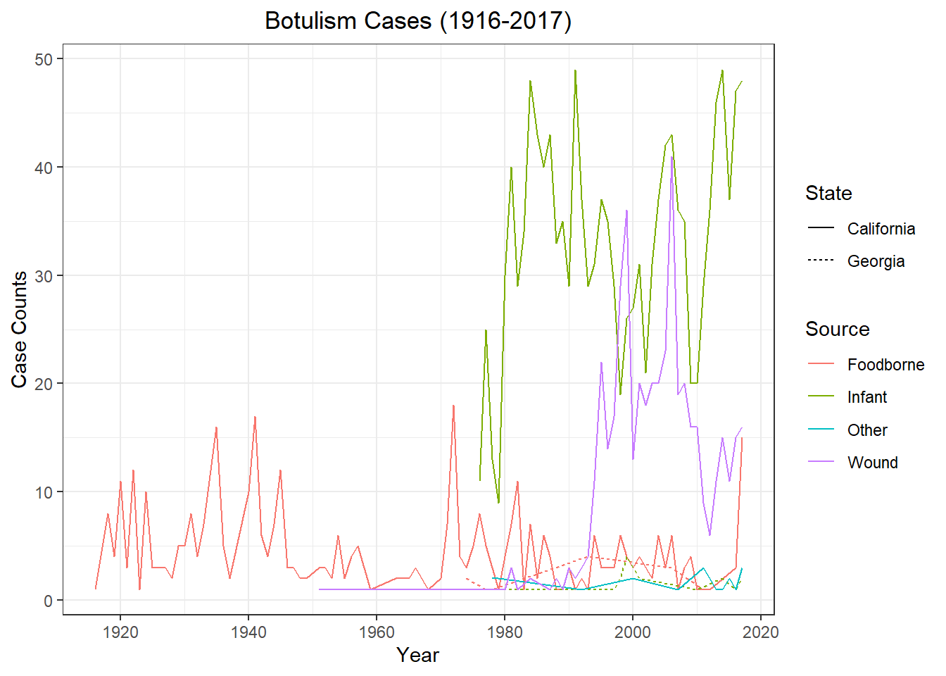
Botulism Cases By State and Source

case_tot %>% ggplot() +geom_line(
  aes(x = Year,
      y = Count,
      color = Source,
      linetype = State)) +
  theme_bw() +
  labs(x = "Year",
       y = "Case Counts",
       title = "Botulism Cases (1916-2017)") +
  theme(plot.title = element_text(hjust = 0.5))

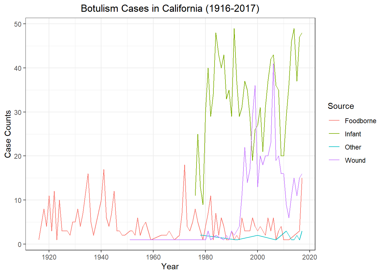
California appears to have a wider range of data collected (across years and different sources). Let’s focus on this State

Let’s look at Botulism counts in California by Source

ca %>% ggplot() +geom_line(
  aes(x = Year,
      y = Count,
      color = Source)) +
  theme_bw() +
  labs(x = "Year",
       y = "Case Counts",
       title = "Botulism Cases in California (1916-2017)") +
  theme(plot.title = element_text(hjust = 0.5))

It wasn’t until the 1970’s that other sources of botulism, such as infant cases, were being detected (Rosow,2015) Let’s look at 1980-2020

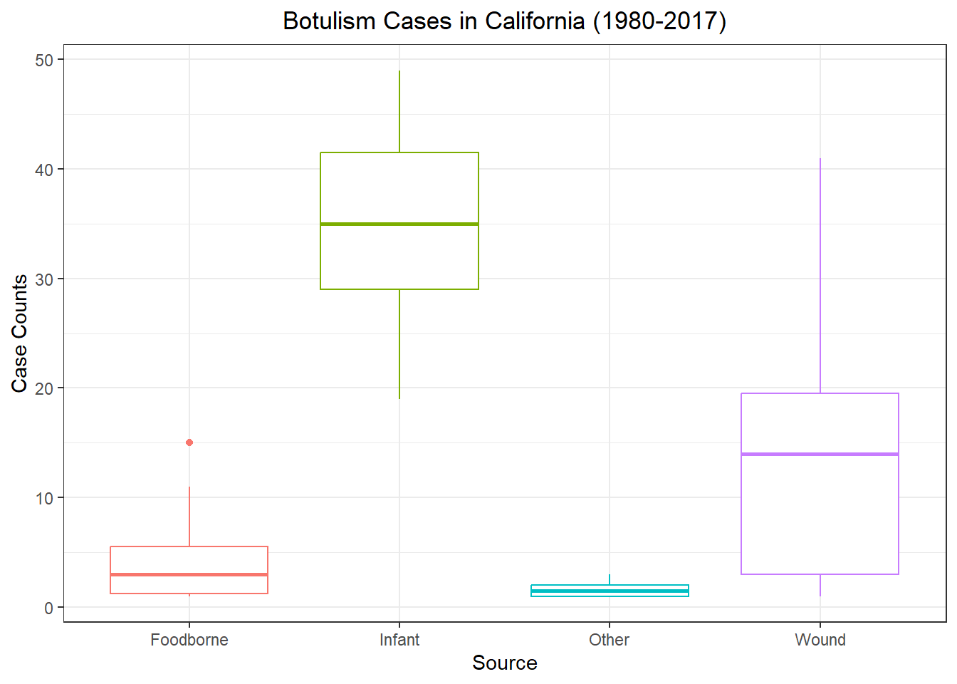
Botulism Cases in California (1980-2017)

ca %>% filter(Year %in% (1980:2020)) %>%
  
ggplot() +geom_boxplot(
  aes(x = Source,
      y = Count,
      color = Source)) +
  theme_bw() +
  labs(y = "Case Counts",
       title = "Botulism Cases in California (1980-2017)") +
  theme(plot.title = element_text(hjust = 0.5),
        legend.position = "none")

Infant cases seem to be the most common. Looking into this, infants are at a higher risk due to their weakened immune system, lack of gastric acidity, and a diminished bacterial flora(Van Horn, 2022). Let’s go back to the strain data and see which strains are most common in infants

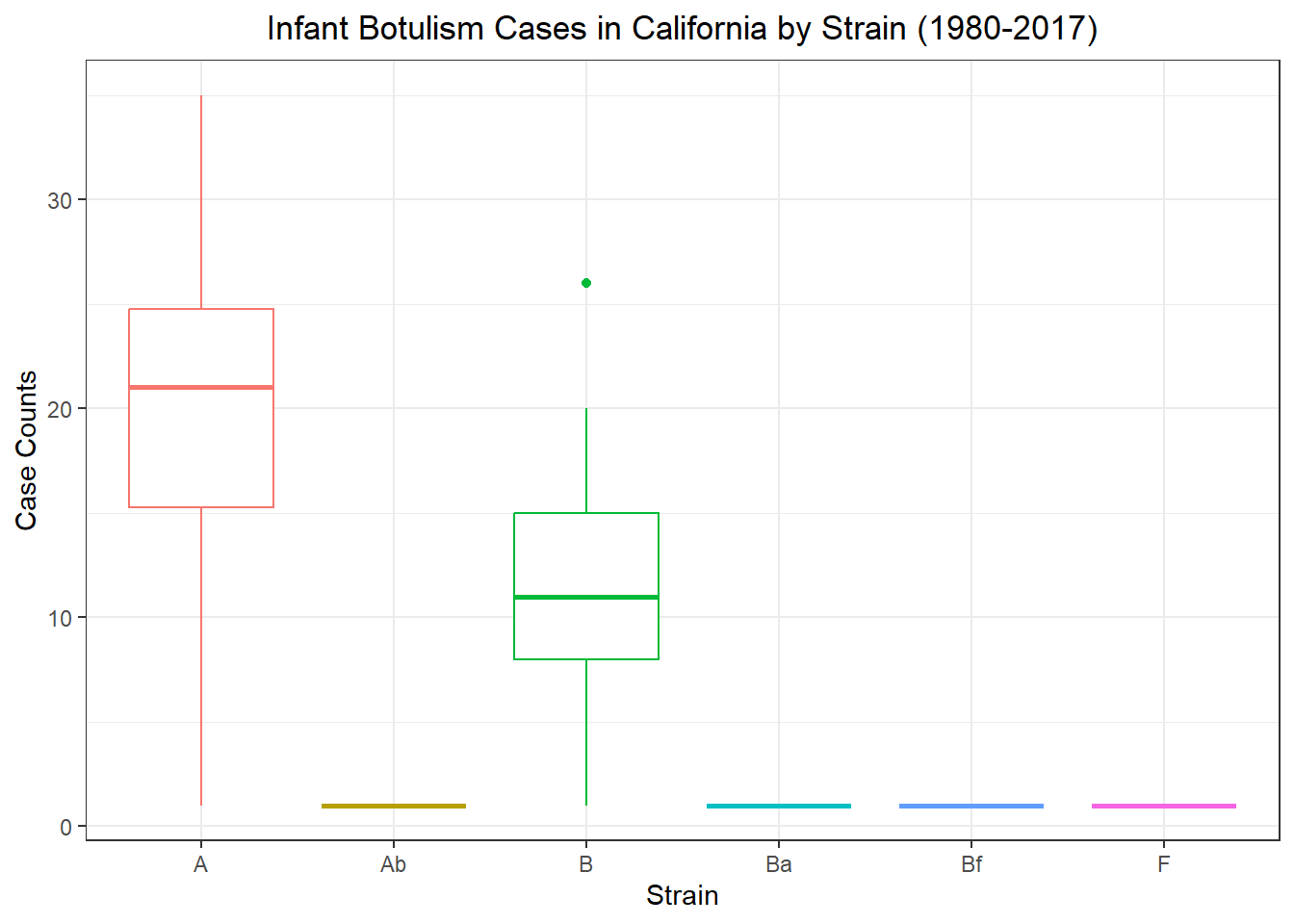
Infant Botulism Cases in California by Strain (1980-2017)

data %>% filter(Year %in% (1980:2020),
                Source %in% "Infant") %>% #Taking original dataset and filtering for 1980-2017 and for infant sources
  
ggplot() +geom_boxplot(
  aes(x = Strain,
      y = Count,
      color = Strain)) +
  theme_bw() +
  labs(y = "Case Counts",
       title = "Infant Botulism Cases in California by Strain (1980-2017)") +
  theme(plot.title = element_text(hjust = 0.5),
       legend.position = "none")

Strain A seems to be the most prevalent in infants followed by Strain B. This can be confirmed at https://www.infantbotulism.org/readings/ib_chapter_6th_edition.pdf