R Coding Exercise

This is the beginning of the loading and checking data exercise where I will install, load, and explore the dslabs package!

NOTE: Use `library()` to list all of the packages installed on my system

Installing packages

install.packages(“dslabs”)

install.packages(“dplyr”)

Loading packages

library ("dplyr")


Attaching package: 'dplyr'

The following objects are masked from 'package:stats':

    filter, lag

The following objects are masked from 'package:base':

    intersect, setdiff, setequal, union

library("dslabs")
library(ggplot2)

What Does the gapminder Dataset Contain?

Look at help file to see what the dataset gapminder contains `help(gapminder)`. Gapminder includes health and income outcomes for 184 countries from 1960 to 2016.

help(gapminder)

starting httpd help server ... done

Overview of data structure

str(gapminder)

'data.frame':   10545 obs. of  9 variables:
 $ country         : Factor w/ 185 levels "Albania","Algeria",..: 1 2 3 4 5 6 7 8 9 10 ...
 $ year            : int  1960 1960 1960 1960 1960 1960 1960 1960 1960 1960 ...
 $ infant_mortality: num  115.4 148.2 208 NA 59.9 ...
 $ life_expectancy : num  62.9 47.5 36 63 65.4 ...
 $ fertility       : num  6.19 7.65 7.32 4.43 3.11 4.55 4.82 3.45 2.7 5.57 ...
 $ population      : num  1636054 11124892 5270844 54681 20619075 ...
 $ gdp             : num  NA 1.38e+10 NA NA 1.08e+11 ...
 $ continent       : Factor w/ 5 levels "Africa","Americas",..: 4 1 1 2 2 3 2 5 4 3 ...
 $ region          : Factor w/ 22 levels "Australia and New Zealand",..: 19 11 10 2 15 21 2 1 22 21 ...

Summary of data

summary(gapminder)

                country           year      infant_mortality life_expectancy
 Albania            :   57   Min.   :1960   Min.   :  1.50   Min.   :13.20  
 Algeria            :   57   1st Qu.:1974   1st Qu.: 16.00   1st Qu.:57.50  
 Angola             :   57   Median :1988   Median : 41.50   Median :67.54  
 Antigua and Barbuda:   57   Mean   :1988   Mean   : 55.31   Mean   :64.81  
 Argentina          :   57   3rd Qu.:2002   3rd Qu.: 85.10   3rd Qu.:73.00  
 Armenia            :   57   Max.   :2016   Max.   :276.90   Max.   :83.90  
 (Other)            :10203                  NA's   :1453                    
   fertility       population             gdp               continent   
 Min.   :0.840   Min.   :3.124e+04   Min.   :4.040e+07   Africa  :2907  
 1st Qu.:2.200   1st Qu.:1.333e+06   1st Qu.:1.846e+09   Americas:2052  
 Median :3.750   Median :5.009e+06   Median :7.794e+09   Asia    :2679  
 Mean   :4.084   Mean   :2.701e+07   Mean   :1.480e+11   Europe  :2223  
 3rd Qu.:6.000   3rd Qu.:1.523e+07   3rd Qu.:5.540e+10   Oceania : 684  
 Max.   :9.220   Max.   :1.376e+09   Max.   :1.174e+13                  
 NA's   :187     NA's   :185         NA's   :2972                       
             region    
 Western Asia   :1026  
 Eastern Africa : 912  
 Western Africa : 912  
 Caribbean      : 741  
 South America  : 684  
 Southern Europe: 684  
 (Other)        :5586

Determining the type of object gapminder is via `class()`

class(gapminder)

[1] "data.frame"

Assigning

I want to create an object (or dataframe) called africadata using an existing dataframe, `gapminder`, then subset gapminder dataframe using the continent column calling Africa (character string to find)

africadata<- gapminder %>% subset(continent=="Africa")

str(africadata)

'data.frame':   2907 obs. of  9 variables:
 $ country         : Factor w/ 185 levels "Albania","Algeria",..: 2 3 18 22 26 27 29 31 32 33 ...
 $ year            : int  1960 1960 1960 1960 1960 1960 1960 1960 1960 1960 ...
 $ infant_mortality: num  148 208 187 116 161 ...
 $ life_expectancy : num  47.5 36 38.3 50.3 35.2 ...
 $ fertility       : num  7.65 7.32 6.28 6.62 6.29 6.95 5.65 6.89 5.84 6.25 ...
 $ population      : num  11124892 5270844 2431620 524029 4829291 ...
 $ gdp             : num  1.38e+10 NA 6.22e+08 1.24e+08 5.97e+08 ...
 $ continent       : Factor w/ 5 levels "Africa","Americas",..: 1 1 1 1 1 1 1 1 1 1 ...
 $ region          : Factor w/ 22 levels "Australia and New Zealand",..: 11 10 20 17 20 5 10 20 10 10 ...

summary (africadata)

         country          year      infant_mortality life_expectancy
 Algeria     :  57   Min.   :1960   Min.   : 11.40   Min.   :13.20  
 Angola      :  57   1st Qu.:1974   1st Qu.: 62.20   1st Qu.:48.23  
 Benin       :  57   Median :1988   Median : 93.40   Median :53.98  
 Botswana    :  57   Mean   :1988   Mean   : 95.12   Mean   :54.38  
 Burkina Faso:  57   3rd Qu.:2002   3rd Qu.:124.70   3rd Qu.:60.10  
 Burundi     :  57   Max.   :2016   Max.   :237.40   Max.   :77.60  
 (Other)     :2565                  NA's   :226                     
   fertility       population             gdp               continent   
 Min.   :1.500   Min.   :    41538   Min.   :4.659e+07   Africa  :2907  
 1st Qu.:5.160   1st Qu.:  1605232   1st Qu.:8.373e+08   Americas:   0  
 Median :6.160   Median :  5570982   Median :2.448e+09   Asia    :   0  
 Mean   :5.851   Mean   : 12235961   Mean   :9.346e+09   Europe  :   0  
 3rd Qu.:6.860   3rd Qu.: 13888152   3rd Qu.:6.552e+09   Oceania :   0  
 Max.   :8.450   Max.   :182201962   Max.   :1.935e+11                  
 NA's   :51      NA's   :51          NA's   :637                        
                       region   
 Eastern Africa           :912  
 Western Africa           :912  
 Middle Africa            :456  
 Northern Africa          :342  
 Southern Africa          :285  
 Australia and New Zealand:  0  
 (Other)                  :  0

Creating new objects

I want to create an object (df) called imle using an existing df, `africadata`, then select 2 columns LE and IM

imle<-africadata %>% select(c("life_expectancy", "infant_mortality"))

ple<- africadata %>% select(c("life_expectancy", "population"))

str(imle)

'data.frame':   2907 obs. of  2 variables:
 $ life_expectancy : num  47.5 36 38.3 50.3 35.2 ...
 $ infant_mortality: num  148 208 187 116 161 ...

summary(imle)

 life_expectancy infant_mortality
 Min.   :13.20   Min.   : 11.40  
 1st Qu.:48.23   1st Qu.: 62.20  
 Median :53.98   Median : 93.40  
 Mean   :54.38   Mean   : 95.12  
 3rd Qu.:60.10   3rd Qu.:124.70  
 Max.   :77.60   Max.   :237.40  
                 NA's   :226

str(ple)

'data.frame':   2907 obs. of  2 variables:
 $ life_expectancy: num  47.5 36 38.3 50.3 35.2 ...
 $ population     : num  11124892 5270844 2431620 524029 4829291 ...

summary(ple)

 life_expectancy   population       
 Min.   :13.20   Min.   :    41538  
 1st Qu.:48.23   1st Qu.:  1605232  
 Median :53.98   Median :  5570982  
 Mean   :54.38   Mean   : 12235961  
 3rd Qu.:60.10   3rd Qu.: 13888152  
 Max.   :77.60   Max.   :182201962  
                 NA's   :51

Plotting

plot_1<- plot(life_expectancy~infant_mortality, data=imle, main="Exercise: Plot 1", ylab= "Life Expectancy", xlab="Infant Mortality")

plot_2<- plot(life_expectancy~population, data=ple, main="Exercise: Plot 2", ylab= "Life Expectancy", xlab="Population", log='x')

Question on data

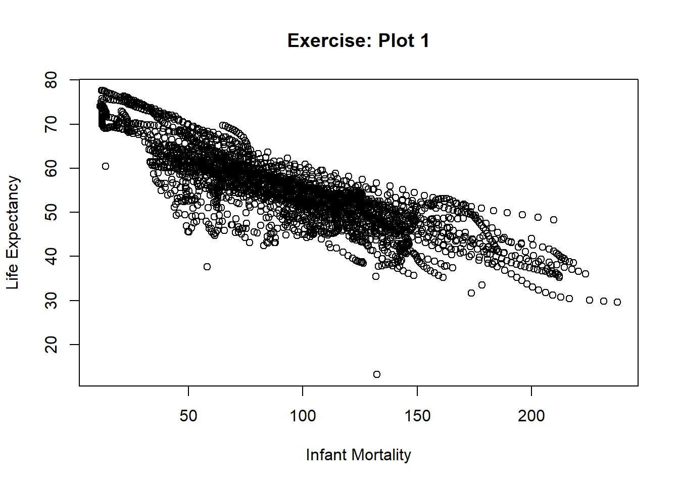
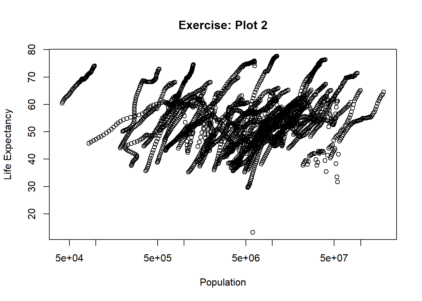
Based on the `africadata` we generated the “clusters” or “streaks” of data seem to be a population in the the same region of Africa over time. Public health strategies that were implemented (e.g., vaccines, clean water, etc.) may have contributed to the increase in life expectancy and a growing population.

More Data Processing

imna<-africadata[is.na(africadata$infant_mortality),]
unique(imna$year)

 [1] 1960 1961 1962 1963 1964 1965 1966 1967 1968 1969 1970 1971 1972 1973 1974
[16] 1975 1976 1977 1978 1979 1980 1981 2016

y2k<- africadata[which(africadata$year=="2000"),]
str(y2k)

'data.frame':   51 obs. of  9 variables:
 $ country         : Factor w/ 185 levels "Albania","Algeria",..: 2 3 18 22 26 27 29 31 32 33 ...
 $ year            : int  2000 2000 2000 2000 2000 2000 2000 2000 2000 2000 ...
 $ infant_mortality: num  33.9 128.3 89.3 52.4 96.2 ...
 $ life_expectancy : num  73.3 52.3 57.2 47.6 52.6 46.7 54.3 68.4 45.3 51.5 ...
 $ fertility       : num  2.51 6.84 5.98 3.41 6.59 7.06 5.62 3.7 5.45 7.35 ...
 $ population      : num  31183658 15058638 6949366 1736579 11607944 ...
 $ gdp             : num  5.48e+10 9.13e+09 2.25e+09 5.63e+09 2.61e+09 ...
 $ continent       : Factor w/ 5 levels "Africa","Americas",..: 1 1 1 1 1 1 1 1 1 1 ...
 $ region          : Factor w/ 22 levels "Australia and New Zealand",..: 11 10 20 17 20 5 10 20 10 10 ...

summary(y2k)

         country        year      infant_mortality life_expectancy
 Algeria     : 1   Min.   :2000   Min.   : 12.30   Min.   :37.60  
 Angola      : 1   1st Qu.:2000   1st Qu.: 60.80   1st Qu.:51.75  
 Benin       : 1   Median :2000   Median : 80.30   Median :54.30  
 Botswana    : 1   Mean   :2000   Mean   : 78.93   Mean   :56.36  
 Burkina Faso: 1   3rd Qu.:2000   3rd Qu.:103.30   3rd Qu.:60.00  
 Burundi     : 1   Max.   :2000   Max.   :143.30   Max.   :75.00  
 (Other)     :45                                                  
   fertility       population             gdp               continent 
 Min.   :1.990   Min.   :    81154   Min.   :2.019e+08   Africa  :51  
 1st Qu.:4.150   1st Qu.:  2304687   1st Qu.:1.274e+09   Americas: 0  
 Median :5.550   Median :  8799165   Median :3.238e+09   Asia    : 0  
 Mean   :5.156   Mean   : 15659800   Mean   :1.155e+10   Europe  : 0  
 3rd Qu.:5.960   3rd Qu.: 17391242   3rd Qu.:8.654e+09   Oceania : 0  
 Max.   :7.730   Max.   :122876723   Max.   :1.329e+11                
                                                                      
                       region  
 Eastern Africa           :16  
 Western Africa           :16  
 Middle Africa            : 8  
 Northern Africa          : 6  
 Southern Africa          : 5  
 Australia and New Zealand: 0  
 (Other)                  : 0

More Plotting

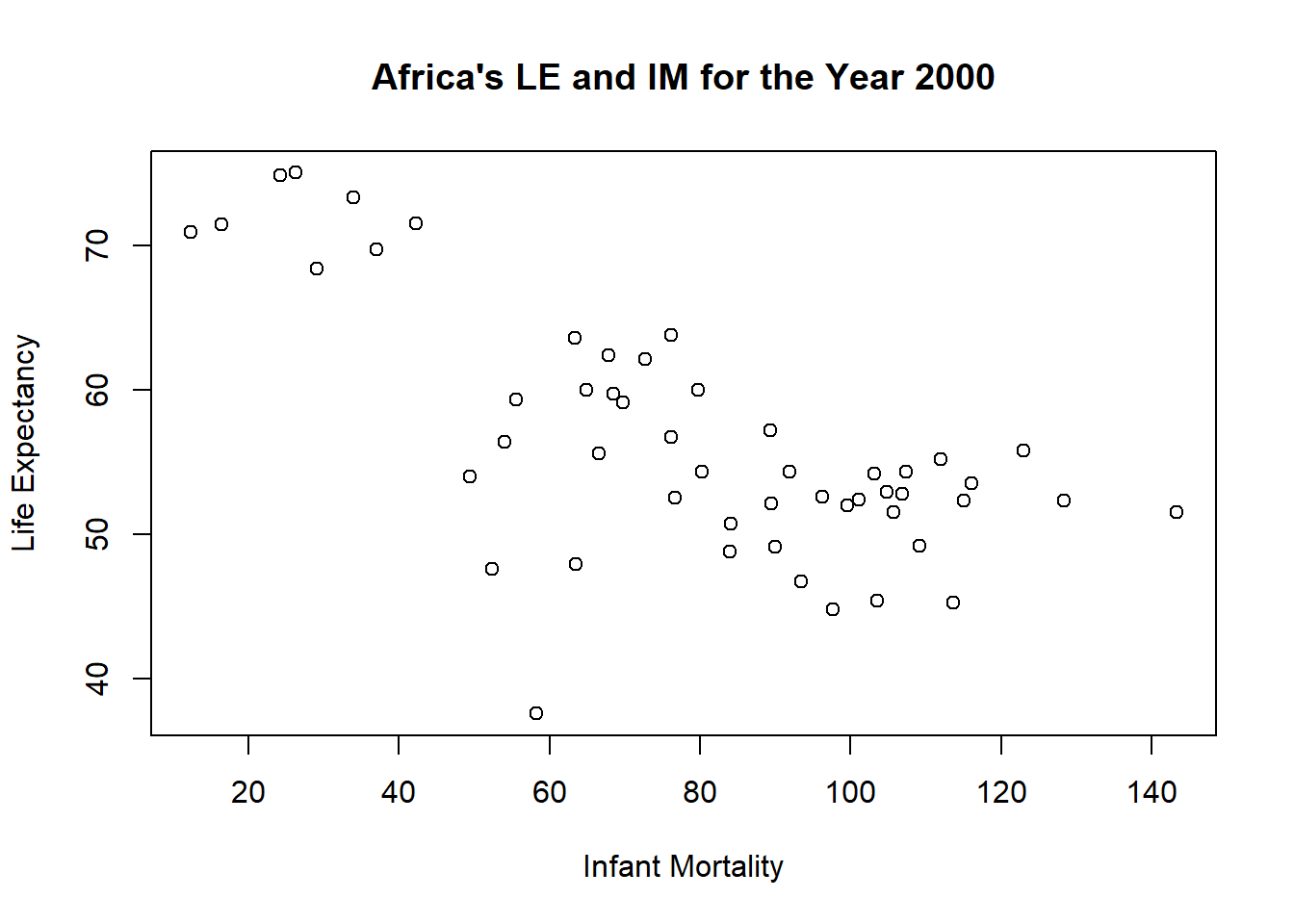
plot_1<- plot(life_expectancy~infant_mortality, data=y2k, main="Africa's LE and IM for the Year 2000", ylab= "Life Expectancy", xlab="Infant Mortality")

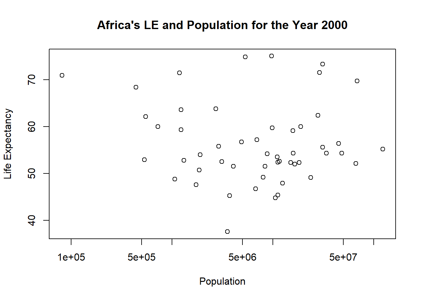
plot_y2k2<- plot(life_expectancy~population, data=y2k, main="Africa's LE and Population for the Year 2000", ylab= "Life Expectancy", xlab="Population", log='x')

A Simple Fit

fit1<-lm(life_expectancy~infant_mortality, data=y2k)
summary(fit1)


Call:
lm(formula = life_expectancy ~ infant_mortality, data = y2k)

Residuals:
     Min       1Q   Median       3Q      Max 
-22.6651  -3.7087   0.9914   4.0408   8.6817 

Coefficients:
                 Estimate Std. Error t value Pr(>|t|)    
(Intercept)      71.29331    2.42611  29.386  < 2e-16 ***
infant_mortality -0.18916    0.02869  -6.594 2.83e-08 ***
---
Signif. codes:  0 '***' 0.001 '**' 0.01 '*' 0.05 '.' 0.1 ' ' 1

Residual standard error: 6.221 on 49 degrees of freedom
Multiple R-squared:  0.4701,    Adjusted R-squared:  0.4593 
F-statistic: 43.48 on 1 and 49 DF,  p-value: 2.826e-08

fit2<-lm(life_expectancy~population, data=y2k)
summary(fit2)


Call:
lm(formula = life_expectancy ~ population, data = y2k)

Residuals:
    Min      1Q  Median      3Q     Max 
-18.429  -4.602  -2.568   3.800  18.802 

Coefficients:
             Estimate Std. Error t value Pr(>|t|)    
(Intercept) 5.593e+01  1.468e+00  38.097   <2e-16 ***
population  2.756e-08  5.459e-08   0.505    0.616    
---
Signif. codes:  0 '***' 0.001 '**' 0.01 '*' 0.05 '.' 0.1 ' ' 1

Residual standard error: 8.524 on 49 degrees of freedom
Multiple R-squared:  0.005176,  Adjusted R-squared:  -0.01513 
F-statistic: 0.2549 on 1 and 49 DF,  p-value: 0.6159

What do the p-values tell us?

Based on the p-values for the given fits, IM as a predictor of LE is said to be statistically significant whereas population as a predictor of LE is said to not statistically significant. But p-values?…

Section by Leah Lariscy

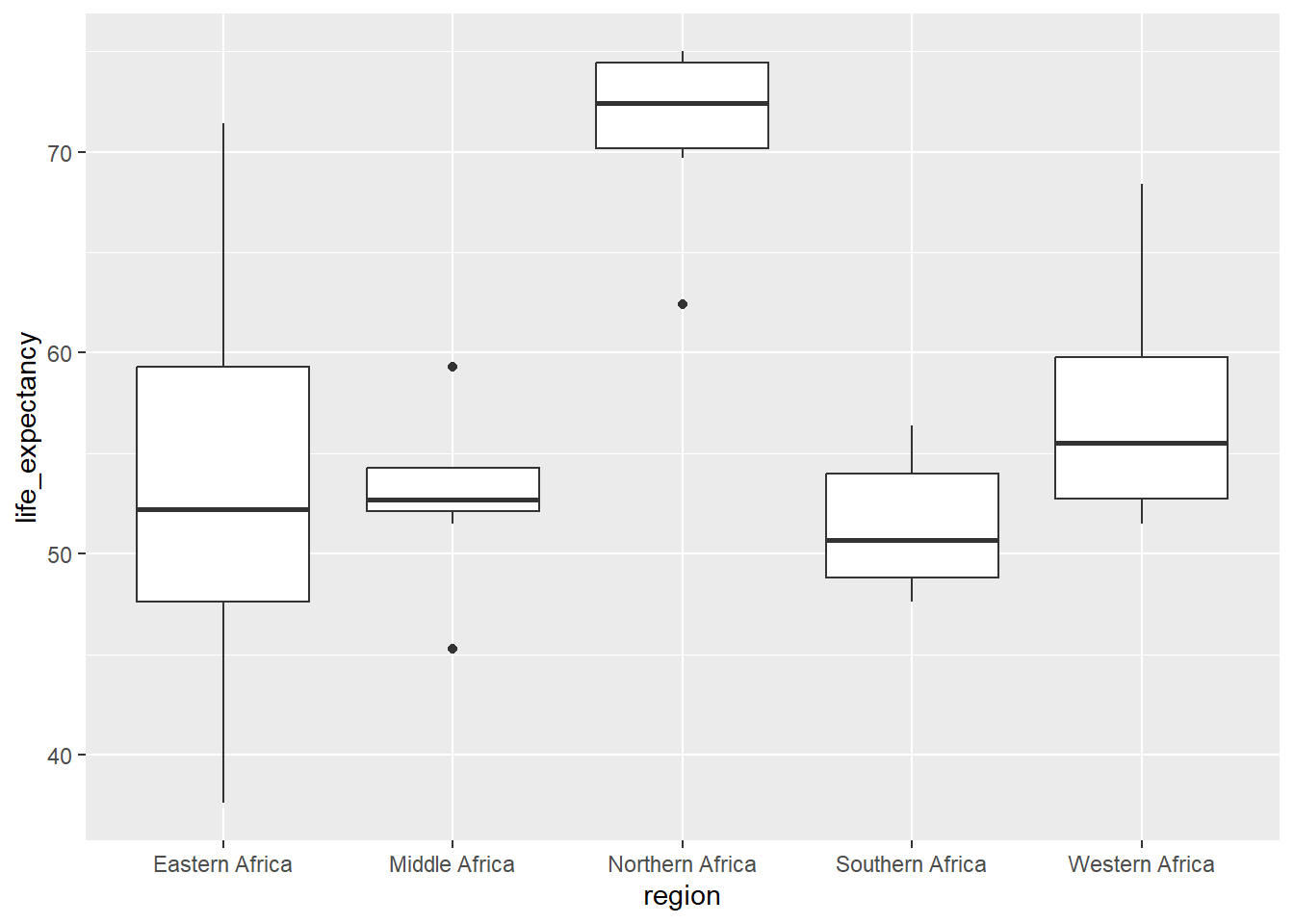
I want to see how LE differs between regions in Africa in 2000. I am going to create a boxplot using `y2k` with `region` on the x-axis and `life_expectancy` on the y-axis

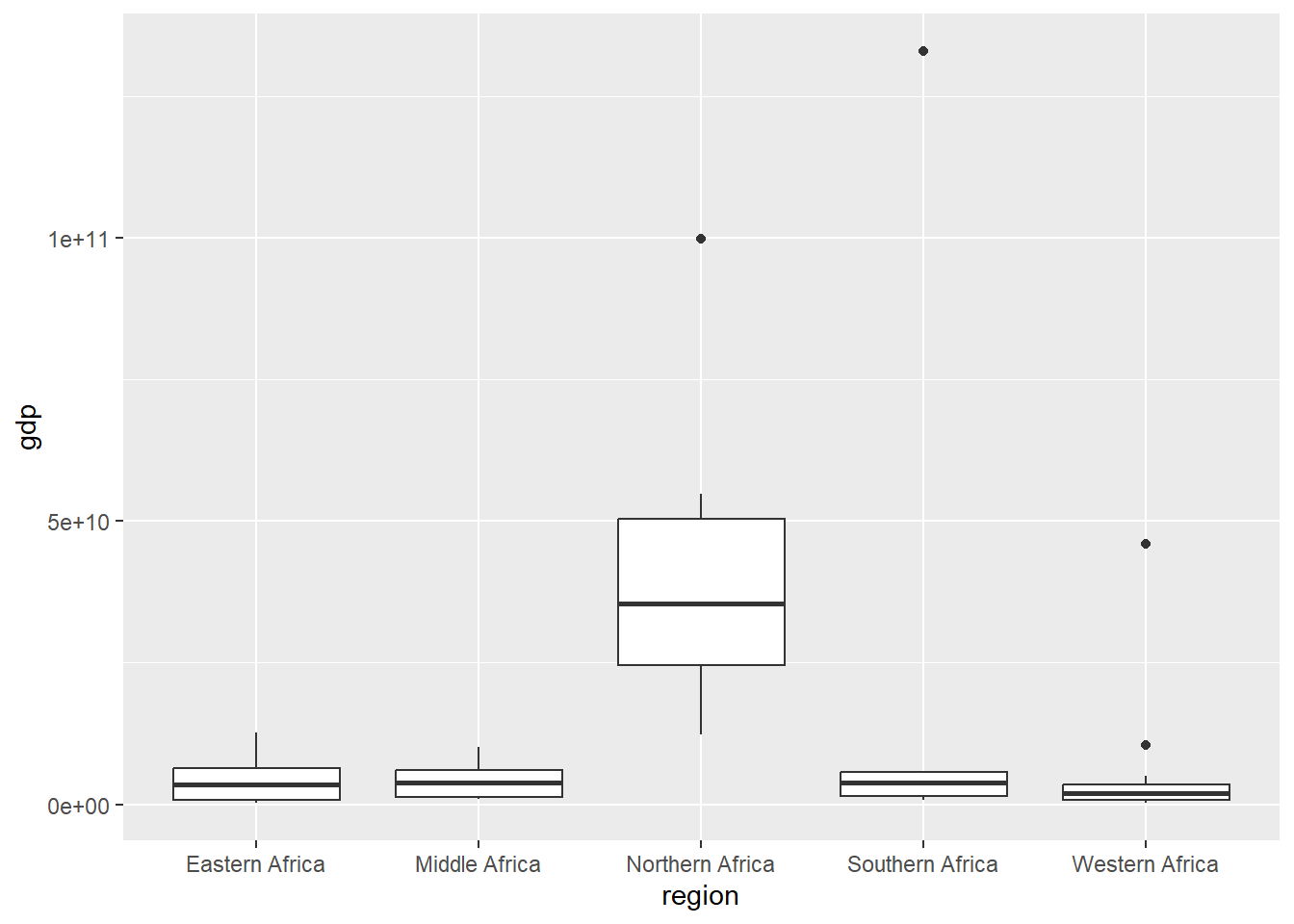
ggplot(data = y2k) + geom_boxplot(aes(region, life_expectancy))

From the plot above, I can tell the life expectancy is significantly higher in Northern Africa than in the rest of the continent. Now I am going to plot `region` vs `gdp` to see if there is a similar trend happening

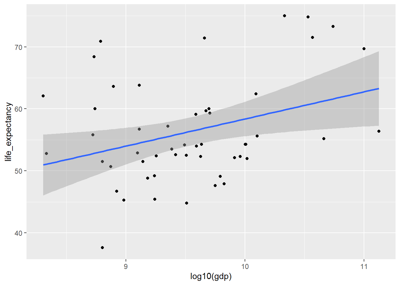
ggplot(data = y2k) + geom_boxplot(aes(region, gdp))

Looking at both of these plots, I am hypothesizing that gdp and life expectancy have a positive correlation aka that gdp is a good predictor for life expectancy. I am now going to plot log10(gdp) vs LE and use `lm`.

ggplot(data = y2k, aes(log10(gdp), life_expectancy)) + geom_point() + geom_smooth(method = "lm")

`geom_smooth()` using formula = 'y ~ x'

y2k_lm <- lm(formula = log10(gdp)~life_expectancy, data = y2k)
summary(y2k_lm)


Call:
lm(formula = log10(gdp) ~ life_expectancy, data = y2k)

Residuals:
     Min       1Q   Median       3Q      Max 
-1.38394 -0.31214  0.00911  0.46180  1.58235 

Coefficients:
                Estimate Std. Error t value Pr(>|t|)    
(Intercept)      8.07684    0.59019  13.685   <2e-16 ***
life_expectancy  0.02596    0.01036   2.507   0.0156 *  
---
Signif. codes:  0 '***' 0.001 '**' 0.01 '*' 0.05 '.' 0.1 ' ' 1

Residual standard error: 0.6196 on 49 degrees of freedom
Multiple R-squared:  0.1137,    Adjusted R-squared:  0.09556 
F-statistic: 6.283 on 1 and 49 DF,  p-value: 0.01556

There is some correlation between gdp and LE across Africa in 2000, but not a strong enough correlation for me to think it is significant.

——————————————–

This section added by RAQUEL FRANCISCO

Install need packages needed and open library

#install.packages('broom')
#install.packages("tidymodels")
library(broom)
library(tidymodels)

── Attaching packages ────────────────────────────────────── tidymodels 1.0.0 ──

✔ dials        1.1.0     ✔ tibble       3.1.8
✔ infer        1.0.4     ✔ tidyr        1.3.0
✔ modeldata    1.1.0     ✔ tune         1.0.1
✔ parsnip      1.0.3     ✔ workflows    1.1.2
✔ purrr        1.0.1     ✔ workflowsets 1.0.0
✔ recipes      1.0.4     ✔ yardstick    1.1.0
✔ rsample      1.1.1

Warning: package 'tidyr' was built under R version 4.2.3

── Conflicts ───────────────────────────────────────── tidymodels_conflicts() ──
✖ purrr::discard() masks scales::discard()
✖ dplyr::filter()  masks stats::filter()
✖ dplyr::lag()     masks stats::lag()
✖ recipes::step()  masks stats::step()
• Search for functions across packages at https://www.tidymodels.org/find/

Use broom package to look at stats differently

Life Exp Vs Infant Mortality

augment(fit1)

# A tibble: 51 × 9
   .rownames life_expect…¹ infan…² .fitted  .resid   .hat .sigma .cooksd .std.…³
   <chr>             <dbl>   <dbl>   <dbl>   <dbl>  <dbl>  <dbl>   <dbl>   <dbl>
 1 7402               73.3    33.9    64.9   8.42  0.0627   6.16 6.54e-2  1.40  
 2 7403               52.3   128.     47.0   5.28  0.0714   6.24 2.98e-2  0.880 
 3 7418               57.2    89.3    54.4   2.80  0.0219   6.27 2.32e-3  0.455 
 4 7422               47.6    52.4    61.4 -13.8   0.0346   5.95 9.10e-2 -2.25  
 5 7426               52.6    96.2    53.1  -0.496 0.0260   6.28 8.69e-5 -0.0807
 6 7427               46.7    93.4    53.6  -6.93  0.0241   6.20 1.57e-2 -1.13  
 7 7429               54.3    91.9    53.9   0.391 0.0232   6.29 4.80e-5  0.0636
 8 7431               68.4    29.1    65.8   2.61  0.0724   6.27 7.41e-3  0.436 
 9 7432               45.3   114.     49.8  -4.50  0.0452   6.25 1.30e-2 -0.741 
10 7433               51.5   106.     51.3   0.201 0.0348   6.29 1.96e-5  0.0329
# … with 41 more rows, and abbreviated variable names ¹life_expectancy,
#   ²infant_mortality, ³.std.resid

glance(fit1)

# A tibble: 1 × 12
  r.squ…¹ adj.r…² sigma stati…³ p.value    df logLik   AIC   BIC devia…⁴ df.re…⁵
    <dbl>   <dbl> <dbl>   <dbl>   <dbl> <dbl>  <dbl> <dbl> <dbl>   <dbl>   <int>
1   0.470   0.459  6.22    43.5 2.83e-8     1  -165.  335.  341.   1896.      49
# … with 1 more variable: nobs <int>, and abbreviated variable names
#   ¹r.squared, ²adj.r.squared, ³statistic, ⁴deviance, ⁵df.residual

tidy(fit1)

# A tibble: 2 × 5
  term             estimate std.error statistic  p.value
  <chr>               <dbl>     <dbl>     <dbl>    <dbl>
1 (Intercept)        71.3      2.43       29.4  8.91e-33
2 infant_mortality   -0.189    0.0287     -6.59 2.83e- 8

Plot by region

ggplot(y2k, aes(life_expectancy,       infant_mortality, color=region)) + geom_point() + stat_smooth(method = "lm", col = "green")

`geom_smooth()` using formula = 'y ~ x'

Life Exp Vs Population

augment(fit2)

# A tibble: 51 × 9
   .rownames life_expecta…¹ popul…² .fitted .resid   .hat .sigma .cooksd .std.…³
   <chr>              <dbl>   <dbl>   <dbl>  <dbl>  <dbl>  <dbl>   <dbl>   <dbl>
 1 7402                73.3  3.12e7    56.8  16.5  0.0295   8.27 5.87e-2   1.97 
 2 7403                52.3  1.51e7    56.3  -4.05 0.0196   8.59 2.30e-3  -0.479
 3 7418                57.2  6.95e6    56.1   1.08 0.0227   8.61 1.90e-4   0.128
 4 7422                47.6  1.74e6    56.0  -8.38 0.0276   8.52 1.41e-2  -0.997
 5 7426                52.6  1.16e7    56.3  -3.65 0.0203   8.60 1.94e-3  -0.433
 6 7427                46.7  6.77e6    56.1  -9.42 0.0229   8.50 1.46e-2  -1.12 
 7 7429                54.3  1.59e7    56.4  -2.07 0.0196   8.61 6.02e-4  -0.245
 8 7431                68.4  4.39e5    55.9  12.5  0.0291   8.42 3.30e-2   1.48 
 9 7432                45.3  3.73e6    56.0 -10.7  0.0254   8.47 2.12e-2  -1.28 
10 7433                51.5  8.34e6    56.2  -4.66 0.0218   8.59 3.41e-3  -0.553
# … with 41 more rows, and abbreviated variable names ¹life_expectancy,
#   ²population, ³.std.resid

glance(fit2)

# A tibble: 1 × 12
  r.squ…¹ adj.r…² sigma stati…³ p.value    df logLik   AIC   BIC devia…⁴ df.re…⁵
    <dbl>   <dbl> <dbl>   <dbl>   <dbl> <dbl>  <dbl> <dbl> <dbl>   <dbl>   <int>
1 0.00518 -0.0151  8.52   0.255   0.616     1  -181.  367.  373.   3560.      49
# … with 1 more variable: nobs <int>, and abbreviated variable names
#   ¹r.squared, ²adj.r.squared, ³statistic, ⁴deviance, ⁵df.residual

tidy(fit2)

# A tibble: 2 × 5
  term             estimate    std.error statistic  p.value
  <chr>               <dbl>        <dbl>     <dbl>    <dbl>
1 (Intercept) 55.9          1.47            38.1   4.51e-38
2 population   0.0000000276 0.0000000546     0.505 6.16e- 1

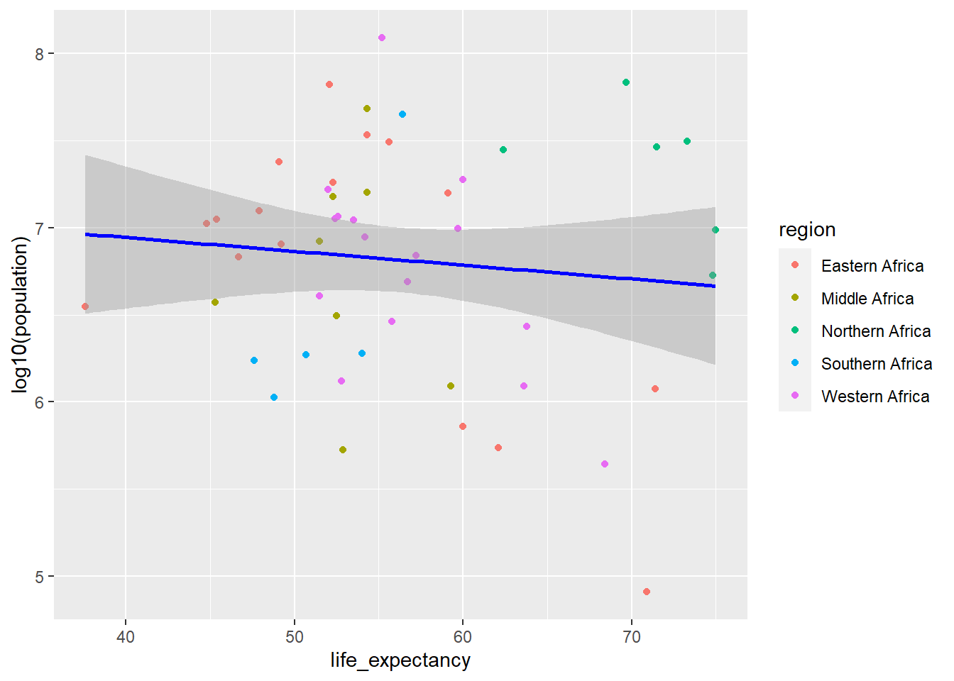
Plot by region

ggplot(y2k, aes(life_expectancy,log10(population), color=region)) + geom_point() + stat_smooth(method = "lm", col = "blue")

`geom_smooth()` using formula = 'y ~ x'

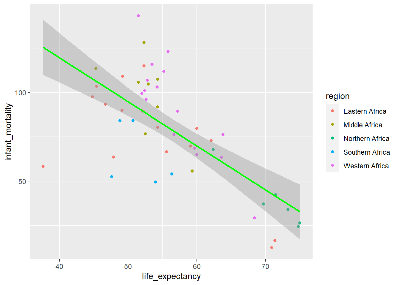
If you look at this raw data it appears that the North African data may be skewing the results. Now lets remove the North African data and see if we get as strong of a correlation…

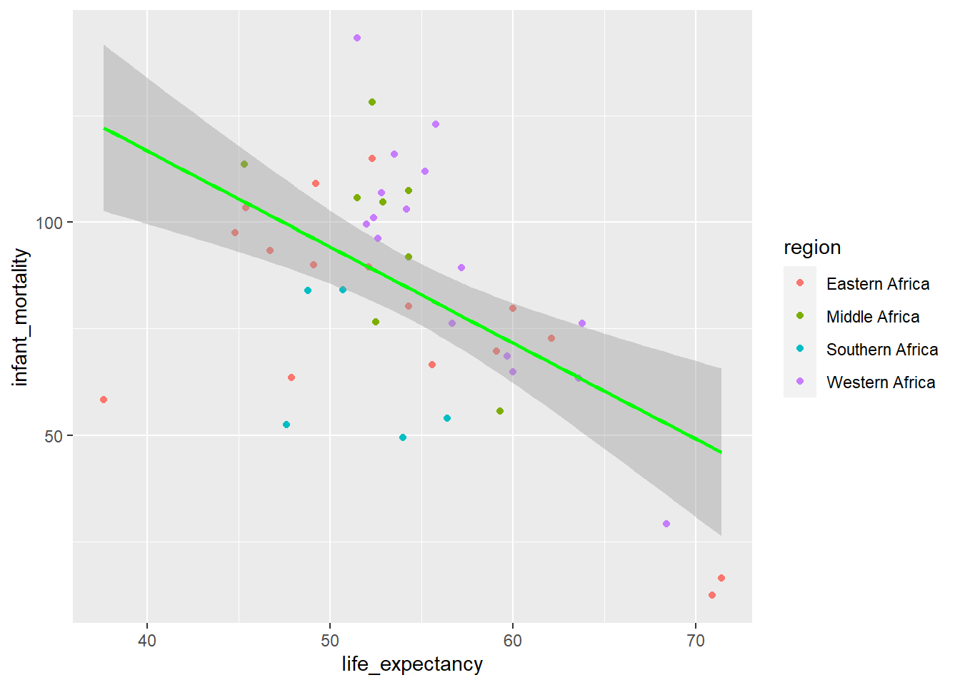
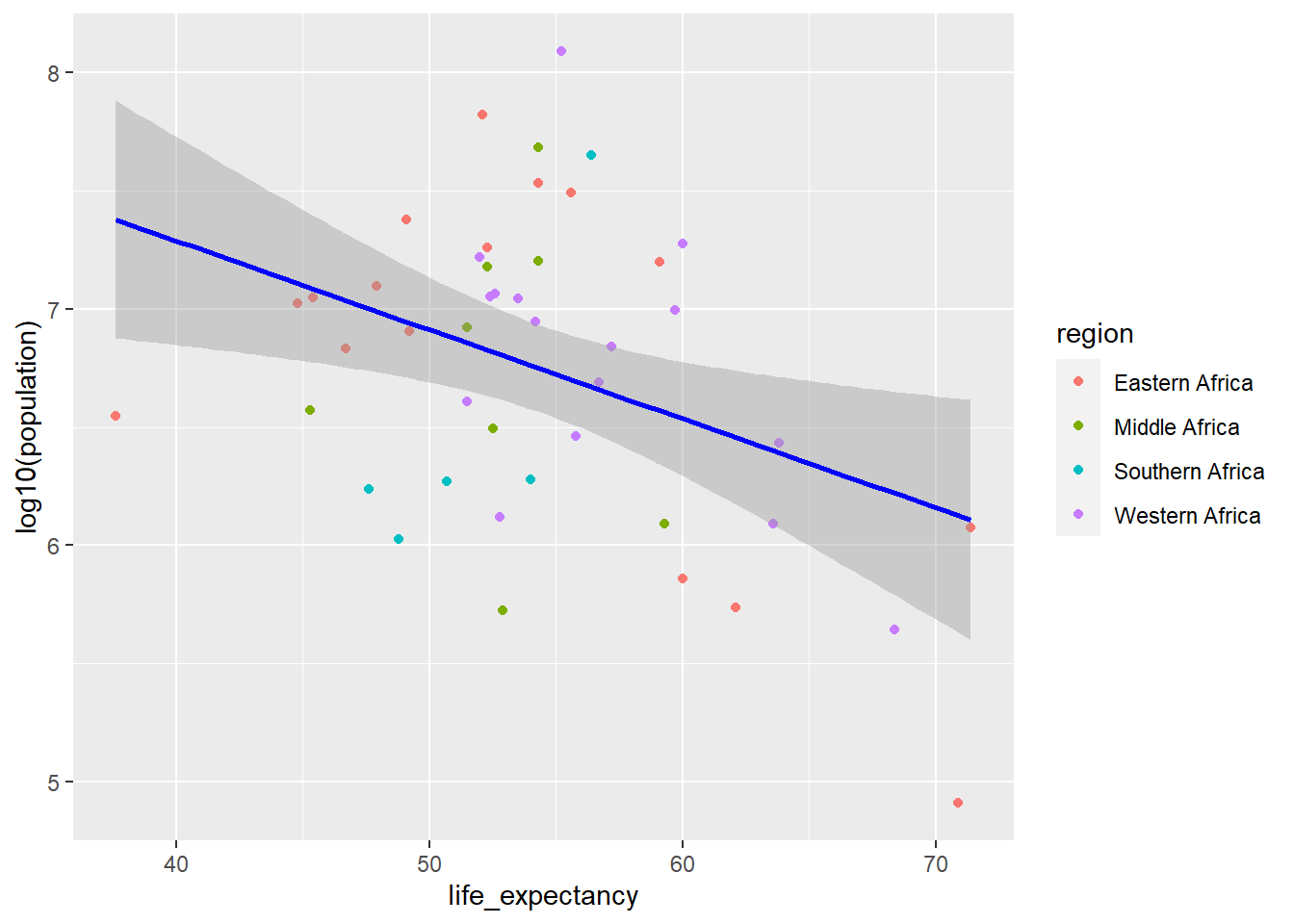
y2kNONA <- y2k %>%
  filter(region == 'Eastern Africa' | region == 'Middle Africa' | region == 'Southern Africa' | region == 'Western Africa')

Data Plots

ggplot(y2kNONA, aes(life_expectancy, infant_mortality, color=region)) + geom_point() + stat_smooth(method = "lm", col = "green")

`geom_smooth()` using formula = 'y ~ x'

ggplot(y2kNONA, aes(life_expectancy,log10(population), color=region)) + geom_point() + stat_smooth(method = "lm", col = "blue")

`geom_smooth()` using formula = 'y ~ x'

Now with Northern Africa removed from the model there does appear a negative relationship between life expectancy and population size, similar to what is seen before and after the removal of Northern Africa from the data when evaluating life expectancy and infant mortality.

This is the beginning of the loading and checking data exercise where I will install, load, and explore the dslabs package!

NOTE: Use library() to list all of the packages installed on my system

Installing packages

Loading packages

What Does the gapminder Dataset Contain?

Look at help file to see what the dataset gapminder contains help(gapminder). Gapminder includes health and income outcomes for 184 countries from 1960 to 2016.

Overview of data structure

Summary of data

Determining the type of object gapminder is via class()

Assigning

I want to create an object (or dataframe) called africadata using an existing dataframe, gapminder, then subset gapminder dataframe using the continent column calling Africa (character string to find)

Creating new objects

I want to create an object (df) called imle using an existing df, africadata, then select 2 columns LE and IM

Plotting

Question on data

More Data Processing

More Plotting

A Simple Fit

What do the p-values tell us?

Based on the p-values for the given fits, IM as a predictor of LE is said to be statistically significant whereas population as a predictor of LE is said to not statistically significant. But p-values?…

Section by Leah Lariscy

I want to see how LE differs between regions in Africa in 2000. I am going to create a boxplot using y2k with region on the x-axis and life_expectancy on the y-axis

From the plot above, I can tell the life expectancy is significantly higher in Northern Africa than in the rest of the continent. Now I am going to plot region vs gdp to see if there is a similar trend happening

Looking at both of these plots, I am hypothesizing that gdp and life expectancy have a positive correlation aka that gdp is a good predictor for life expectancy. I am now going to plot log10(gdp) vs LE and use lm.

There is some correlation between gdp and LE across Africa in 2000, but not a strong enough correlation for me to think it is significant.

——————————————–

This section added by RAQUEL FRANCISCO

Install need packages needed and open library

Use broom package to look at stats differently

Life Exp Vs Infant Mortality

Plot by region

Life Exp Vs Population

Plot by region

If you look at this raw data it appears that the North African data may be skewing the results. Now lets remove the North African data and see if we get as strong of a correlation…

Data Plots

Now with Northern Africa removed from the model there does appear a negative relationship between life expectancy and population size, similar to what is seen before and after the removal of Northern Africa from the data when evaluating life expectancy and infant mortality.

NOTE: Use `library()` to list all of the packages installed on my system

Look at help file to see what the dataset gapminder contains `help(gapminder)`. Gapminder includes health and income outcomes for 184 countries from 1960 to 2016.

Determining the type of object gapminder is via `class()`

I want to create an object (or dataframe) called africadata using an existing dataframe, `gapminder`, then subset gapminder dataframe using the continent column calling Africa (character string to find)

I want to create an object (df) called imle using an existing df, `africadata`, then select 2 columns LE and IM

I want to see how LE differs between regions in Africa in 2000. I am going to create a boxplot using `y2k` with `region` on the x-axis and `life_expectancy` on the y-axis

From the plot above, I can tell the life expectancy is significantly higher in Northern Africa than in the rest of the continent. Now I am going to plot `region` vs `gdp` to see if there is a similar trend happening

Looking at both of these plots, I am hypothesizing that gdp and life expectancy have a positive correlation aka that gdp is a good predictor for life expectancy. I am now going to plot log10(gdp) vs LE and use `lm`.